Make Your Machine Learning Predictions More Robust With This Trick

Understanding Test Time Augmentation.

Scarce data can be problematic for training a deep learning model.

Luckily, data augmentation exists.

Data augmentation is the practice of increasing your training data by applying operations like flipping, cropping, or scaling.

But, did you know you can also apply data augmentation on your test data?

What is Test Time Augmentation

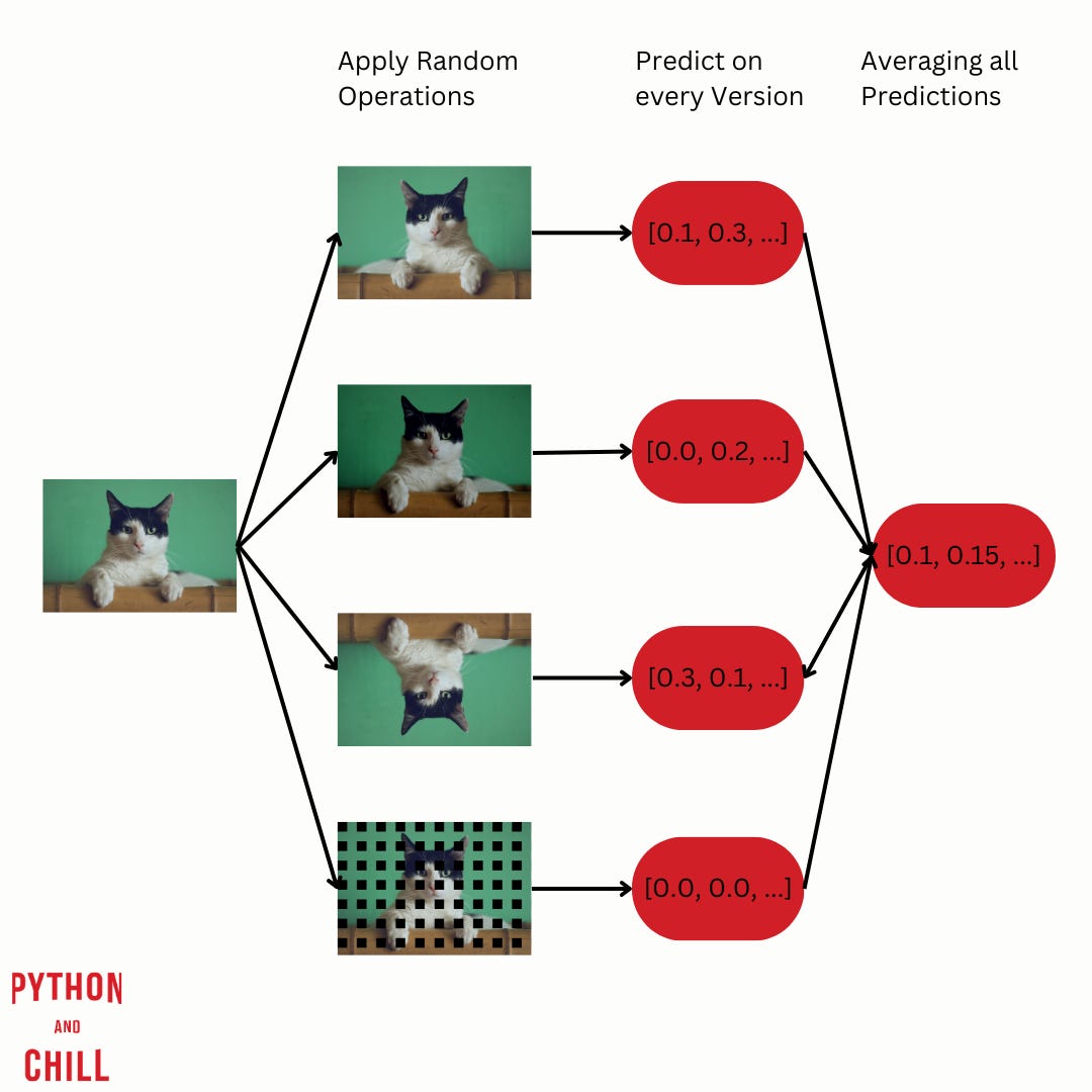
Test Time Augmentation (TTA) refers to a technique where you apply data augmentation during testing.

At inference time, instead of showing a test example one time to your model, you show multiple versions of the test example by applying different random operations.

Your model makes predictions for every version of the test example.

Finally, the predictions will be averaged and outputted.

TTA essentially creates an ensemble of predictions by considering multiple augmented versions of the same input, which leads to a more robust final prediction.

In this novel paper, the authors even prove that TTA is less than or equal to the average error of an original model.

So, where is the catch?

Downside of TTA

As you can imagine, the inference time increases with TTA.

Multiple versions of the images will be created, and the model has to predict for every version.

So, when a low inference time is important to you, think twice about TTA.

Implementation in Python

You see, to understand TTA you don’t need a PHD.

And the implementation is easy too.

For our small example, we will use Keras + TensorFlow for our CV model.

For augmentation, we use Albumentations. Albumentations makes it easy to apply a wide range of augmentation techniques.

So, install the requirements:

albumentations==2.0.3
keras==3.8.0
tensorflow==2.18.0
opencv-python==4.11.0.86
numpy==1.26.4

import numpy as np
import tensorflow as tf
from tensorflow import keras
import albumentations as A
from albumentations.core.composition import OneOf
import cv2

def augment_image(image):
    transform = A.Compose([
        OneOf([
            A.HorizontalFlip(p=1),
            A.VerticalFlip(p=1),
            A.Rotate(limit=30, p=1),
            A.Transpose(p=1)
        ], p=1),
    ])
    augmented = transform(image=image)
    return augmented["image"]

def load_and_preprocess_image(image_path, target_size=(224, 224)):
    image = cv2.imread(image_path)
    image = cv2.cvtColor(image, cv2.COLOR_BGR2RGB)
    image = cv2.resize(image, target_size)
    image = image.astype(np.float32) / 255.0
    return image

def generate_tta_images(image, num_augmentations=5):
    images = [image]
    for _ in range(num_augmentations):
        aug_img = augment_image(image)
        images.append(aug_img)
    return np.array(images)

model = keras.applications.MobileNetV2(weights='imagenet', include_top=True)

def tta_predict(model, image_path, num_augmentations=5):
    image = load_and_preprocess_image(image_path)
    tta_images = generate_tta_images(image, num_augmentations)
    
    tta_images = np.array([cv2.resize(img, (224, 224)) for img in tta_images])

    predictions = []
    for img in tta_images:
        img = np.expand_dims(img, axis=0)
        pred = model.predict(img)
        predictions.append(pred)
    
    avg_prediction = np.mean(predictions, axis=0).squeeze()
    
    return avg_prediction

image_path = "cat.png"
final_prediction = tta_predict(model, image_path)

decoded_prediction = keras.applications.mobilenet_v2.decode_predictions(final_prediction[np.newaxis, :], top=3)
print(decoded_prediction) 

Let’s go step by step:

1. augment_image() is responsible for apply a selected transformation on the image.

2. load_and_preprocess_image() prepares the image for the CV model we will use (MobileNet), which needs an image size of 224 x 224.

3. generate_tta_images() will generate `n` transformed images for our model to predict at test time.

4. tta_predict() runs the predictions on the transformed images.

That’s it. With this simple set up, you can apply TTA to your images.

Conclusion

You learned about a powerful yet not widely used technique named TTA. It stands out for images where the model is unsure since it gets multiple versions to make a prediction and the error will be averaged at the end.